There is an important mathematical constant called \(e\) which plays a useful role in calculus and the sciences. The activity below is intended to help you discover one interpretation of the value of this constant.
The graph below shows the exponential function \(f(x) = b^x\) along with the so-called tangent line at the \(y\)-intercept. This line is the best-fit of a linear function to the exponential function’s graph at the point \((0,1)\text{.}\) It just “touches” the curve at this point. Move the slider to adjust the base \(b\) of the exponential function and observe how it affects the slope of the tangent line equation \(y = mx + 1\text{.}\)
Move the slider to find the largest value of \(b\) that results in a slope of the tangent which is less than \(1\text{.}\) Record this value of \(b\text{.}\)
Move the slider to find the smallest value of \(b\) that results in a slope of the tangent which is greater than \(1\text{.}\) Record this value of \(b\text{.}\)
There must is a special value of \(b\) called \(e\) for which the slope of the tangent is exactly \(1\text{.}\) In what interval is this special number \(e\) in?
There is a real number \(e\) for which the slope of the tangent line to \(y = e^x\) at \((0,1)\) is exactly \(1\text{.}\) We call \(e\) the natural base and the function \(y = e^x\) the natural exponential function.
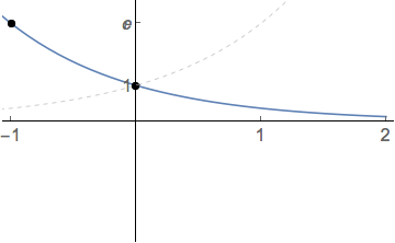
In fact, \(e\approx 2.718 \gt 1\) is an irrational number and at best can be only approximated with a finite number of digits. The graph of the natural exponential function grows exponentially with domain \((-\infty,\infty)\) and range \((0,\infty)\text{.}\) Like all exponential functions, it has a \(y\)-intercept at \((0,1)\text{.}\) The graph decays to the left towards its horizontal asymptote \(y = 0\text{.}\)
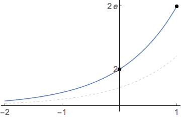
The graph of \(\displaystyle y = 2e^{x}\) is obtained by stretching the graph of \(y=e^{x}\) vertically by a factor or 2. This changes the \(y\)-intercept, but does not change the horizontal asymptote.
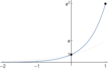
The graph of \(\displaystyle y = e^{2x}\) is obtained by compressing the graph of \(y=e^x\) horizontally by a factor of 2. This does not change the \(y\)-intercept nor the horizontal asymptote, but it does increase the rate at which the graph grows.
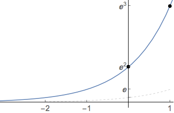
The graph of \(\displaystyle y = e^{x+2}\) is obtained by translating the graph of \(y=e^x\) two units to the left. This changes the \(y\)-intercept, but not the overall shape of the graph.
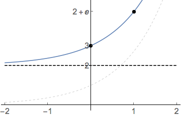
The graph of \(\displaystyle y = e^{x}+2\) is obtained by translating the graph of \(y=e^x\) two units up. This changes the \(y\)-intercept to \(0,3\) and the horizontal asymptote to \(y=2\text{.}\)